Algorithms and Data Structures

Algorithms, Object Oriented Programming, Data Structures and Software Engineering

what are the main things a developer should be familiar with, in order to make an efficient software?

• Efficient Algorithms to perform tasks

• data Structures to hold and manipulate data

• OOPS to make a secure, stable, scalable and reusable code

• Software Engineering to do above said tasks in the best possible way

Data Structures

Data Structures are the abstract or virtual data holding containers which define a scheme for how to store data in memory and process it. There already exist many data structures like linked lists, stacks, queues, trees, graphs and many more. A data structure must be chosen wisely by keeping in mind the complexity and type of data to store and the data manipulations and operations to be performed on it. Data structures are ways in which data is arranged in your computer’s memory (or stored on disk). And Algorithms are the procedures, a software program uses to manipulate the data in these structures.

Algorithms

An algorithm in layman’s terms is a set of stepwise instructions written in a simple easy to understand ways to perform any complex task efficiently. In computer field these instructions follow some conventions and rules also. These English written instructions are later on converted into compatible source code using a programming language and suitable editors.

OOPS

Object Oriented Programming Struct is the latest software design methodology which emerged due to the rising incapability of structural or procedural designing techniques to handle large and complex problems. OOPS changed the way a programmer looks at the problem now. Instead of considering operations for software development, OOPS design process focus on the data and then the operation to be performed on it. OOP relates the problem at hand with the actual reality and real objects having own properties and functions. Objects and classes play an important role in implementing object orientation. Object oriented programming (OOP) offers compelling advantages over the old-fashioned procedural approach, and is quickly replacing it for serious program development.

Objects in a Nutshell The idea of objects arose in the programming community as a solution to the problems with procedural languages. An object contains both methods and variables. A class is a specification—a blueprint—for one or more objects.

Software Engineering

With just Bits & Bytes - you can build entire businesses and industries over it, and that too in a virtual world, nothing physical at all. This is the beauty of Software Engineering ! Software engineering is a study concerned with designing and implementing large and complex software projects. Software engineering defines the software development phases and steps to design, develop, implement, maintain and test the software and is applicable from the very beginning of the application development process and to the end of it. Software engineering mentions the use of extensive tools to perform each task. Information gathering is the primary and most important phase of a software development process. As in each phase we are gathering information only. Like before making an application, we decide what algorithms to implement and which data structure to use and this decision is made possible only after gathering the information about all data structures and algorithms. Similarly during maintenance and testing phase also we are continuously gathering info to find errors and areas of maintenance. Software engineering is the study of ways to create large and complex computer programs, involving many programmers. It focuses on the overall design of the programs and on the creation of that design from the needs of the end users. Software engineering is concerned with the life cycle of a software project, which includes specification, design, verification, coding, testing, production, and maintenance. Software engineering is rather abstract and is difficult to grasp until you’ve been involved yourself in a large project.

What happens to the code on collective application of above mentioned concepts?

When the knowledge of all of these subjects is collectively applied, we get an optimized, complete and efficient code. By optimized, complete and efficient software code I mean, that the source code is complete, almost free from bugs and errors, of lower complexity or fast (algorithms prove their point here), scalable, secure (scalability and security comes from object oriented design) and easily reusable (inheritance plays an important role in code reuse).

How to apply them collectively?

Whenever we’re given a software project or product to build we are provided with some raw information and the type of data which would be encountered while in the software development phase and also the operations and data manipulations to be done on the data. So our first step should be to choose the appropriate data structure which could easily handle the enormous amount of such data and complex operations performed on this data. In order to make operations we’ve to devise an algorithm. Mind it, an object oriented algorithm is the new trend.

But before implementing all these steps, what essentially required in prior is the research. As a famous saying in the programming world suggests: “The sooner you start to code, the longer the program will take“

So an extensive exhaustive research is always required before writing the actual code. A research to find out which data structure is the best, a research to deduct an efficient object oriented algorithm with least complexity and a research to find out how and what classes should be made and what methods/functions the objects of those classes should perform. This is done with the help of software engineering tools and concepts.

Algorithms, data structures and the object oriented struct are somewhat closely related to each other and the concepts are applied while the actual code writing process. Almost every serious programmer spend about a year on these subjects. Software engineering plays no role in writing the code as such but helps in deciding what to write i.e what algorithms to apply, which data structure to use and what parts of the program should obey object oriented rules and where to use functional or procedural programming methodologies. That is why software engineering is studied in separation to them and mostly ignored by the developers.

An introduction to data structures

This part describes about some commonly used data structures and their applications in the real programming world. So here’s the brief guide to data structures and abstract data types (ADT’s)

Computer system is mainly used as a data manipulation system. Elementary data can be represented in these forms:

• Data

• data items

• data structures

Data structures are mainly used to accomplish the following tasks on the given data:

• data representation

• data storage

• data organisation

• data processing

• data management

All these are data manipulation processes only. Data structures let us combine data of different types and process them together. It refers to a named group of data of different types which can be processed as a single unit. A data structure has well defined set of operations, behaviour and properties.

Situations in which they’re useful are classified into three categories:

• Real-world data storage

• Programmer’s tools

• Modelling

Things to keep in mind while designing a data structure:

• logical picture

• data representation method

• operations to be applied

In computer science, a data structure is a particular way of storing and organizing data in a computer so that it can be used efficiently. Different kinds of data structures are suited to different kinds of applications, and some are highly specialized to specific tasks. For example, B-trees are particularly well-suited for implementation of databases, while compiler implementations usually use hash tables to look up identifiers. Data structures are used in almost every program or software system. Data structures provide a means to manage huge amounts of data efficiently, such as large databases and internet indexing services. Usually, efficient data structures are a key to designing efficient algorithms. Some formal design methods and programming languages emphasize data structures, rather than algorithms, as the key organizing factor in software design.

Basic principles

Data structures are generally based on the ability of a computer to fetch and store data at any place in its memory, specified by an address—a bit string that can be itself stored in memory and manipulated by the program. Thus the record and array data structures are based on computing the addresses of data items with arithmetic operations; while the linked data structures are based on storing addresses of data items within the structure itself. Many data structures use both principles, sometimes combined in non-trivial ways (as in XOR linking) The implementation of a data structure usually requires writing a set of procedures that create and manipulate instances of that structure. The efficiency of a data structure cannot be analyzed separately from those operations. This observation motivates the theoretical concept of an abstract data type, a data structure that is defined indirectly by the operations that may be performed on it, and the mathematical properties of those operations (including their space and time cost).

Common data structures

Common data structures include: array, linked list, hash-table, heap, Tree (Binary Tree, B-tree, red-black tree), stack, and queue.

Language support

Most assembly languages and some low-level languages, such as BCPL, lack support for data structures. Many high-level programming languages, and some higher-level assembly languages, such as MASM, on the other hand, have special syntax or other built-in support for certain data structures, such as vectors (one-dimensional arrays) in the C language or multi-dimensional arrays in Pascal. Most programming languages feature some sorts of library mechanism that allows data structure implementations to be reused by different programs. Modern languages usually come with standard libraries that implement the most common data structures. Examples are the C++ Standard Template Library, the Java Collections Framework, and Microsoft’s .NET Framework. Modern languages also generally support modular programming, the separation between the interface of a library module and its implementation. Some provide opaque data types that allow clients to hide implementation details. Object-oriented programming languages, such as C++, Java and .NET Framework use classes for this purpose.

Data structures may be simple or compound or linear and non linear

Arrays and structure come under simple category while linked lists, stacks, queues are categorised into non-linear data structures which are of compound nature as well. Trees and graphs are also the non-linear compound data structures.

Some Common Data Structures

Arrays

Stacks A stack can be used to check whether parentheses, braces, and brackets are balanced in a computer. A stack is also a handy aid for algorithms applied to certain complex data structures. Stack plays a vital role in parsing (analysing) arithmetic expressions such as 3*(4+5). Most microprocessors use a stack-based architecture. When a method is called, its return address and arguments are pushed onto a stack, and when it returns, they’re popped off. The stack operations are built into the microprocessor. Some older pocket calculators used a stack-based architecture. Instead of entering arithmetic expressions using parentheses, you pushed intermediate results onto a stack.

Binary Trees It is used to help traverse the nodes of a tree.

Graphs Searching the vertices of a graph (a technique that can be used to find your way out of a maze).

Linked lists

Queues They’re also used to model real-world situations such as people waiting in line at a bank, airplanes waiting to take off, or data packets waiting to be transmitted over the Internet. There are various queues quietly doing their job in your computer’s (or the network’s) operating system. There’s a printer queue where print jobs wait for the Queues printer to be available. A queue also stores keystroke data as you type at the keyboard. This way, if you’re using a word processor but the computer is briefly doing something else when you hit a key, the keystroke won’t be lost; it waits in the queue until the word processor has time to read it. Using a queue guarantees the keystrokes stay in order until they can be processed.

Priority queue Like ordinary queues, priority queues are used in various ways in certain computer systems. In a preemptive multitasking operating system, for example, programs may be placed in a priority queue so the highest-priority program is the next one to receive a time-slice that allows it to execute.

Trees

Stacks, queues and priority queues are the programmer’s data srructures.

static memory allocation occurs at the compile time hence fixed size data types

dynamic memory allocation takes place during the run time hence data structures can be of variable size

contagious and non contagious memory allocation

free pool allocation

garbage collection

Algorithms + data structures = programs

Pseudocode

source code

algorithm

byte code

overflow and underflow

Abstract data type ADT can be defined as a set of values and set of operations where implementation part is hidden. ADT is a mathematical model for a certain class of data types of one or more programming language that have similar semantics.

common operations done on data structures

traversal

searching

sorting

insertion

deletion

query

Algorithms and Complexity Analysis

This part of the document describes about the commonly used algorithms a programmer must be familiar with and the concepts to construct fast and efficient algorithms for any problem.

After reading this, you will be able to distinguish between the following terms and will have a better understanding of the concept of complexity analysis and algorithms. • big O notation • asymptotic behaviour • worst-case analysis • sorting techniques and their complexities

Introduction The term analysis of algorithms is used to describe approaches to the study of the performance of algorithms. Algorithm complexity is just a way to formally measure how fast a program or algorithm runs, so it really is quite pragmatic. We already know there are tools to measure how fast a program runs. There are programs called profilers which measure running time in milliseconds and can help us optimize our code by spotting bottlenecks. While this is a useful tool, it isn’t really relevant to algorithm complexity. Algorithm complexity is something designed to compare two algorithms at the idea level — ignoring low-level details such as the implementation programming language, the hardware the algorithm runs on, or the instruction set of the given CPU. We want to compare algorithms in terms of just what they are: Ideas of how something is computed. Counting milliseconds won’t help us in that. It’s quite possible that a bad algorithm written in a low-level programming language such as assembly runs much quicker than a good algorithm written in a high-level programming language such as Python or Ruby. So it’s time to define what a “better algorithm” really is.

As algorithms are programs that perform just a computation, and not other things computers often do such as networking tasks or user input and output, complexity analysis allows us to measure how fast a program is when it performs computations. Examples of operations that are purely computational include:

• numerical floating-point operations such as addition and multiplication

• searching within a database that fits in RAM for a given value

• running a regular expression pattern match on a string.

Clearly, computation is ubiquitous in computer programs. Complexity analysis is also a tool that allows us to explain how an algorithm behaves as the input grows larger. If we feed it a different input, how will the algorithm behave? If our algorithm takes 1 second to run for an input of size 1000, how will it behave if I double the input size? Will it run just as fast, half as fast, or four times slower? In practical programming, this is important as it allows us to predict how our algorithm will behave when the input data becomes larger. For example, if we’ve made an algorithm for a web application that works well with 1000 users and measure its running time, using algorithm complexity analysis we can have a pretty good idea of what will happen once we get 2000 users instead. For algorithmic competitions, complexity analysis gives us insight about how long our code will run for the largest test cases that are used to test our program’s correctness. So if we’ve measured our program’s behaviour for a small input, we can get a good idea of how it will behave for larger inputs.

Algorithm In mathematics and computer science, an algorithm is a step-by-step procedure for calculations. Algorithms are used for calculation, data processing, and automated reasoning. An algorithm is an effective method expressed as a finite list of well-defined instructions for calculating a function.

How do we compare algorithms ?

(1) Compare execution times? Not good: times are specific to a particular computer

(2) Count the number of statements executed?
Not good: number of statements vary with the programming language as well as the style of the individual programmer.

We need to define a number of objective measures. Ideal Solution: Express running time as a function of the input size n (i.e., f(n)). Compare different functions corresponding to running times. To compare two algorithms with running times f(n) and g(n) given, we need a rough measure that characterizes how fast each function grows. Such an analysis is independent of machine time, programming style, etc.

Counting instructions The maximum element in an array can be looked up using a simple piece of code written in javascript. Given an input array A of size n:

var M = A[ 0 ];
for ( var i = 0; i < n; ++i ) {
if ( A[ i ] >= M ) {
M = A[ i ];
}
}

Now, the first thing we’ll do is count how many fundamental instructions this piece of code executes. As we analyse this piece of code, we want to break it up into simple instructions; things that can be executed by the CPU directly - or close to that. We’ll assume our processor can execute the following operations as one instruction each:

• Assigning a value to a variable

• Looking up the value of a particular element in an array

• Comparing two values

• Incrementing a value

• Basic arithmetic operations such as addition and multiplication

We’ll assume branching (the choice between if and else parts of code after the if condition has been evaluated) occurs instantly and won’t count these instructions. In the above code, the first line of code is: var M = A[ 0 ];

This requires 2 instructions: One for looking up A[ 0 ] and one for assigning the value to M (we’re assuming that n is always at least 1). These two instructions are always required by the algorithm, regardless of the value of n. The for loop initialization code also has to always run. This gives us two more instructions; an assignment and a comparison: i = 0; i < n;

These will run before the first for loop iteration. After each for loop iteration, we need two more instructions to run, an increment of i and a comparison to check if we’ll stay in the loop: ++i; i < n;

So, if we ignore the loop body, the number of instructions this algorithm needs is 4 + 2n. That is, 4 instructions at the beginning of the for loop and 2 instructions at the end of each iteration of which we have n. We can now define a mathematical function f( n ) that, given an n, gives us the number of instructions the algorithm needs. For an empty for body, we have f( n ) = 4 + 2n.

Kinds of Analysis

Worst-case maximum time of an algorithm on any input of size n The worst case analysis of an algorithm provides an upper bound on running time and an absolute guarantee that the algorithm would not run longer, no matter what the inputs are.

Average-case The expected time of algorithm over all inputs of size n. Need assumption of statistical distribution of inputs. The average case analysis provides the prediction about the running time and assumes that the input is random.

Best-case cheat with a slow algorithm that works fast on a particular input. The best case analysis of an algorithm provides a lower bound on running time. Input is the one for which the algorithm runs the fastest. Lower bound < running time < upper bound

Worst-case analysis Now, looking at the for body, we have an array lookup operation and a comparison that happen always: if ( A[ i ] >= M ) { … That’s two instructions right there. But the if body may run or may not run, depending on what the array values actually are. If it happens to be so that A[ i ] >= M, then we’ll run these two additional instructions — an array lookup and an assignment: M = A[ i ] But now we can’t define an f( n ) as easily, because our number of instructions doesn’t depend solely on n but also on our input. For example, for A = [ 1, 2, 3, 4 ] the algorithm will need more instructions than for A = [ 4, 3, 2, 1 ]. When analysing algorithms, we often consider the worst-case scenario. What’s the worst that can happen for our algorithm? When does our algorithm need the most instructions to complete? In this case, it is when we have an array in increasing order such as A = [ 1, 2, 3, 4 ]. In that case, M needs to be replaced every single time and so that yields the most instructions. Computer scientists have a fancy name for that and they call it worst-case analysis; that’s nothing more than just considering the case when we’re the most unlucky. So, in the worst case, we have 4 instructions to run within the for body, so we have f( n ) = 4 + 2n + 4n = 6n + 4. This function f, given a problem size n, gives us the number of instructions that would be needed in the worst-case.

Asymptotic behavior

In our function, 6n + 4, we have two terms: 6n and 4. In complexity analysis we only care about what happens to the instruction-counting function as the program input (n) grows large. This really goes along with the previous ideas of “worst-case scenario” behaviour: We’re interested in how our algorithm behaves when treated badly; when it’s challenged to do something hard. Notice that this is really useful when comparing algorithms. If an algorithm beats another algorithm for a large input, it’s most probably true that the faster algorithm remains faster when given an easier, smaller input. From the terms that we are considering, we’ll drop all the terms that grow slowly and only keep the ones that grow fast as n becomes larger. Clearly 4 remains a 4 as n grows larger, but 6n grows larger and larger, so it tends to matter more and more for larger problems. Therefore, the first thing we will do is drop the 4 and keep the function as f( n ) = 6n. This makes sense if you think about it, as the 4 is simply an “initialization constant”. Different programming languages may require a different time to set up. For example, Java needs some time to initialize its virtual machine. Since we’re ignoring programming language differences, it only makes sense to ignore this value. The second thing we’ll ignore is the constant multiplier in front of n, and so our function will become f( n ) = n. As you can see this simplifies things quite a lot. Again, it makes some sense to drop this multiplicative constant if we think about how different programming languages compile. The “array lookup” statement in one language may compile to different instructions in different programming languages. For example, in C, doing A[ i ] does not include a check that i is within the declared array size, while in Pascal it does. So, the following Pascal code: M := A[ i ] Is the equivalent of the following in C: if ( i >= 0 && i < n ) { M = A[ i ]; } So it’s reasonable to expect that different programming languages will yield different factors when we count their instructions. In our example in which we are using a dumb compiler for Pascal that is oblivious of possible optimizations, Pascal requires 3 instructions for each array access instead of the 1 instruction C requires. Dropping this factor goes along the lines of ignoring the differences between particular programming languages and compilers and only analysing the idea of the algorithm itself. This filter of “dropping all factors” and of “keeping the largest growing term” as described above is what we call asymptotic behaviour. So the asymptotic behaviour of f( n ) = 2n + 8 is described by the function f( n ) = n. Mathematically speaking, what we’re saying here is that we’re interested in the limit of function f as n tends to infinity. In a strict mathematical setting, we would not be able to drop the constants in the limit; but for computer science purposes, we want to do that for the reasons described above. Now let us find the asymptotic behaviour of the following example functions by dropping the constant factors and by keeping the terms that grow the fastest.

1. f( n ) = 5n + 12 gives f( n ) = n. By using the exact same reasoning as above.
2. f( n ) = 109 gives f( n ) = 1. We’re dropping the multiplier 109 * 1, but we still have to put a 1 here to indicate that this function has a non-zero value.
3. f( n ) = n2 + 3n + 112 gives f( n ) = n2 Here, n2 grows larger than 3n for sufficiently large n, so we’re keeping that.
4. f( n ) = n3 + 1999n + 1337 gives f( n ) = n3 Even though the factor in front of n is quite large, we can still find a large enough n so that n3 is bigger than 1999n. As we’re interested in the behaviour for very large values of n, we only keep n^3 Some more examples
5. f( n ) = n6 + 3n
6. f( n ) = 2n + 12
7. f( n ) = 3n + 2n
8. f( n ) = nn + n

If you’re having trouble with one of the above, plug in some large n and see which term is bigger. Asymptotic curves of some common functions. Don’t forget to check the values of each function for large values of input x.

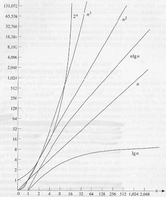
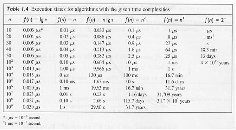
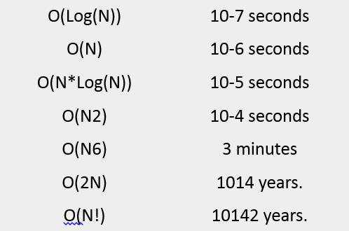
Execution time for common functions Complexity So what this is telling us is that since we can drop all these decorative constants, it’s pretty easy to tell the asymptotic behaviour of the instruction-counting function of a program. In fact, any program that doesn’t have any loops will have f( n ) = 1, since the number of instructions it needs is just a constant (unless it uses recursion; see below). Any program with a single loop which goes from 1 to n will have f( n ) = n, since it will do a constant number of instructions before the loop, a constant number of instructions after the loop, and a constant number of instructions within the loop which all run n times. This should now be much easier and less tedious than counting individual instructions, so let’s take a look at a couple of examples to get familiar with this. The following PHP program checks to see if a particular value exists within an array A of size n:

<?php
$exists = false;
for ( $i = 0; $i < n; ++$i ) {
if ( $A[ $i ] == $value ) {
$exists = true;
break;

This method of searching for a value within an array is called linear search. This is a reasonable name, as this program has f( n ) = n . You may notice that there’s a “break” statement here that may make the program terminate sooner, even after a single iteration. But recall that we’re interested in the worst-case scenario, which for this program is for the array A to not contain the value. So we still have f( n ) = n.

Systematically analyse the number of instructions the above PHP program needs with respect to n in the worst-case to find f( n ), similarly to how we analysed our first Javascript program. Then verify that, asymptotically, we have f( n ) = n.

Let’s look at a Python program which adds two array elements together to produce a sum which it stores in another variable: v = a[ 0 ] + a[ 1 ] Here we have a constant number of instructions, so we have f( n ) = 1. The following program in C++ checks to see if a vector (a form of array) named A of size n contains the same two values anywhere within it: bool duplicate = false; for ( int i = 0; i < n; ++i ) { for ( int j = 0; j < n; ++j ) { if ( i != j && A[ i ] == A[ j ] ) { duplicate = true; break; } } if ( duplicate ) { break; } }

As here we have two nested loops within each other, we’ll have an asymptotic behaviour described by f( n ) = n^2(n-square).

Note: Simple programs can be analysed by counting the nested loops of the program. A single loop over n items yields f( n ) = n. A loop within a loop yields f( n ) = n2. A loop within a loop within a loop yields f( n ) = n3. If we have a program that calls a function within a loop and we know the number of instructions the called function performs, it’s easy to determine the number of instructions of the whole program. Indeed, let’s take a look at this C example: int i; for ( i = 0; i < n; ++i ) { f( n ); } If we know that f( n ) is a function that performs exactly n instructions, we can then know that the number of instructions of the whole program is asymptotically n2, as the function is called exactly n times.

note: Given a series of for loops that are sequential, the slowest of them determines the asymptotic behaviour of the program. Two nested loops followed by a single loop is asymptotically the same as the nested loops alone, because the nested loops dominate the simple loop.

Now, let’s switch over to the fancy notation that computer scientists use. When we’ve figured out the exact such f asymptotically, we’ll say that our program is Θ( f( n ) ). For example, the above programs are Θ( 1 ), Θ( n2 ) and Θ( n2 ) respectively. Θ( n ) is pronounced “theta of n”. Sometimes we say that f( n ), the original function counting the instructions including the constants, is Θ( something ). For example, we may say that f( n ) = 2n is a function that is Θ( n ) — nothing new here. We can also write 2n ∈ Θ( n ), which is pronounced as “two n is theta of n”. Don’t get confused about this notation: All it’s saying is that if we’ve counted the number of instructions a program needs and those are 2n, then the asymptotic behaviour of our algorithm is described by n, which we found by dropping the constants. Given this notation, the following are some true mathematical statements:

1. n6 + 3n ∈ Θ( n6 )
2. 2n + 12 ∈ Θ( 2n )
3. 3n + 2n ∈ Θ( 3n )
4. nn + n ∈ Θ( nn )

We call this function, i.e. what we put within Θ( here ), the time complexity or just complexity of our algorithm. So an algorithm with Θ( n ) is of complexity n. We also have special names for Θ( 1 ), Θ( n ), Θ( n2 ) and Θ( log( n ) ) because they occur very often. We say that a Θ( 1 ) algorithm is a constant-time algorithm, Θ( n ) is linear, Θ( n2 ) is quadratic and Θ( log( n ) ) is logarithmic.

note: Programs with a bigger Θ run slower than programs with a smaller Θ.

Time/Space trade off A programmer usually has a choice of data structures and algorithms to use. Choosing the best one for a particular job involves, among other factors, two important measures: Time Complexity: how much time will the program take? Space Complexity: how much storage will the program need? A programmer will sometimes seek a trade-off between space and time complexity. For example, a programmer might choose a data structure that requires a lot of storage in order to reduce the computation time. There is an element of art in making such trade-offs, but the programmer must make the choice from an informed point of view. The programmer must have some verifiable basis on which to make the selection of a data structure or algorithm. Complexity analysis provides such a basis. Complexity refers to the rate at which the storage or time grows as a function of the problem size. The absolute growth depends on the machine used to execute the program, the compiler used to construct the program, and many other factors. We would like to have a way of describing the inherent complexity of a program (or piece of a program), independent of machine/compiler considerations. This means that we must not try to describe the absolute time or storage needed. We must instead concentrate on a “proportionality” approach, expressing the complexity in terms of its relationship to some known function. This type of analysis is known as asymptotic analysis. Asymptotic analysis is based on the idea that as the problem size grows, the complexity can be described as a simple proportionality to some known function. This idea is incorporated in the “Big Oh” notation for asymptotic performance.

Definition: T(n) = O(f(n)) if and only if there are constants c0 and n0 such that T(n) <= c0 f(n) for all n >= n0. The expression “T(n) = O(f(n))” is read as “T of n is in Big Oh of f of n.” Big Oh is sometimes said to describe an “upper-bound” on the complexity. Other forms of asymptotic analysis (“Big Omega”, “Little Oh”, “Theta”) are similar in spirit to Big Oh.

Big-O notation Now, it’s sometimes true that it will be hard to figure out exactly the behaviour of an algorithm in this fashion as we did above, especially for more complex examples. However, we will be able to say that the behaviour of our algorithm will never exceed a certain bound. This will make life easier for us, as we won’t have to specify exactly how fast our algorithm runs, even when ignoring constants the way we did before. All we’ll have to do is find a certain bound. This is explained easily with an example. A famous problem computer scientists use for teaching algorithms is the sorting problem. In the sorting problem, an array A of size n is given and we are asked to write a program that sorts this array. This problem is interesting because it is a pragmatic problem in real systems. For example, a file explorer needs to sort the files it displays by name so that the user can navigate them with ease. Sorting is also interesting because there are many algorithms to solve it, some of which are worse than others. It’s also an easy problem to define and to explain. So let’s write a piece of code that sorts an array. Here is an inefficient way to implement sorting an array in Ruby. (Of course, Ruby supports sorting arrays using build-in functions which you should use instead, and which are certainly faster than what we’ll see here. But this is here for illustration purposes.) b = [] n.times do m = a[ 0 ] mi = 0 a.each_with_index do |element, i| if element < m m = element mi = i end end a.delete_at( mi ) b « m end

This method is called selection sort. It finds the minimum of our array (the array is denoted a above, while the minimum value is denoted m and mi is its index), puts it at the end of a new array (in our case b), and removes it from the original array. Then it finds the minimum between the remaining values of our original array, appends that to our new array so that it now contains two elements, and removes it from our original array. It continues this process until all items have been removed from the original and have been inserted into the new array, which means that the array has been sorted. In this example, we can see that we have two nested loops. The outer loop runs n times, and the inner loop runs once for each element of the array a. While the array a initially has n items, we remove one array item in each iteration. So the inner loop repeats n times during the first iteration of the outer loop, then n - 1 times, then n - 2 times and so forth, until the last iteration of the outer loop during which it only runs once. It’s a little harder to evaluate the complexity of this program, as we’d have to figure out the sum 1 + 2 + … + (n - 1) + n. But we can for sure find an “upper bound” for it. That is, we can alter our program to make it worse than it is and then find the complexity of that new program that we derived. If we can find the complexity of the worse program that we’ve constructed, then we know that our original program is at most that bad, or maybe better. That way, if we find out a pretty good complexity for our altered program, which is worse than our original, we can know that our original program will have a pretty good complexity too – either as good as our altered program or even better. Let’s now think of the way to edit this example program to make it easier to figure out its complexity. But let’s keep in mind that we can only make it worse, i.e. make it take up more instructions, so that our estimate is meaningful for our original program. Clearly we can alter the inner loop of the program to always repeat exactly n times instead of a varying number of times. Some of these repetitions will be useless, but it will help us analyse the complexity of the resulting algorithm. If we make this simple change, then the new algorithm that we’ve constructed is clearly Θ( n2 ), because we have two nested loops where each repeats exactly n times. If that is so, we say that the original algorithm is O( n2 ). O( n2 ) is pronounced “big oh of n squared”. What this says is that our program is asymptotically no worse than n2. It may even be better than that, or it may be the same as that. By the way, if our program is indeed Θ( n2 ), we can still say that it’s O( n2 ). To help you realize that, imagine altering the original program in a way that doesn’t change it much, but still makes it a little worse, such as adding a meaningless instruction at the beginning of the program. Doing this will alter the instruction-counting function by a simple constant, which is ignored when it comes to asymptotic behaviour. So a program that is Θ( n2 ) is also O( n2 ). But a program that is O( n2 ) may not be Θ( n2 ). For example, any program that is Θ( n ) is also O( n2 ) in addition to being O( n ). If we imagine the that a Θ( n ) program is a simple for loop that repeats n times, we can make it worse by wrapping it in another for loop which repeats n times as well, thus producing a program with f( n ) = n2. To generalize this, any program that is Θ( a ) is O( b ) when b is worse than a. Notice that our alteration to the program doesn’t need to give us a program that is actually meaningful or equivalent to our original program. It only needs to perform more instructions than the original for a given n. All we’re using it for is counting instructions, not actually solving our problem. So, saying that our program is O( n2 ) is being on the safe side: We’ve analysed our algorithm, and we’ve found that it’s never worse than n2. But it could be that it’s in fact n2. This gives us a good estimate of how fast our program runs. Let’s go through a few examples to help you familiarize yourself with this new notation.

Find out which of the following are true:

1. A Θ( n ) algorithm is O( n )
2. A Θ( n ) algorithm is O( n2 )
3. A Θ( n2 ) algorithm is O( n3 )
4. A Θ( n ) algorithm is O( 1 )
5. A O( 1 ) algorithm is Θ( 1 )
6. A O( n ) algorithm is Θ( 1 ) Solutions
7. We know that this is true as our original program was Θ( n ). We can achieve O( n ) without altering our program at all.
8. As n2 is worse than n, this is true.
9. As n3 is worse than n2, this is true.
10. As 1 is not worse than n, this is false. If a program takes n instructions asymptotically (a linear number of instructions), we can’t make it worse and have it take only 1 instruction asymptotically (a constant number of instructions).
11. This is true as the two complexities are the same.
12. This may or may not be true depending on the algorithm. In the general case it’s false. If an algorithm is Θ( 1 ), then it certainly is O( n ). But if it’s O( n ) then it may not be Θ( 1 ). For example, a Θ( n ) algorithm is O( n ) but not Θ( 1 ).

Use an arithmetic progression sum to prove that the above program is not only O( n2 ) but also Θ( n2 ). Because the O-complexity of an algorithm gives an upper bound for the actual complexity of an algorithm, while Θ gives the actual complexity of an algorithm, we sometimes say that the Θ gives us a tight bound. If we know that we’ve found a complexity bound that is not tight, we can also use a lower-case o to denote that. For example, if an algorithm is Θ( n ), then its tight complexity is n. Then this algorithm is both O( n ) and O( n2 ). As the algorithm is Θ( n ), the O( n ) bound is a tight one. But the O( n2 ) bound is not tight, and so we can write that the algorithm is o( n2 ), which is pronounced “small o of n squared” to illustrate that we know our bound is not tight. It’s better if we can find tight bounds for our algorithms, as these give us more information about how our algorithm behaves, but it’s not always easy to do.

Determine which of the following bounds are tight bounds and which are not tight bounds. Check to see if any bounds may be wrong. Use o( notation ) to illustrate the bounds that are not tight.

1. A Θ( n ) algorithm for which we found a O( n ) upper bound.
2. A Θ( n2 ) algorithm for which we found a O( n3 ) upper bound.
3. A Θ( 1 ) algorithm for which we found an O( n ) upper bound.
4. A Θ( n ) algorithm for which we found an O( 1 ) upper bound.
5. A Θ( n ) algorithm for which we found an O( 2n ) upper bound. Solution
6. In this case, the Θ complexity and the O complexity are the same, so the bound is tight.
7. Here we see that the O complexity is of a larger scale than the Θ complexity so this bound is not tight. Indeed, a bound of O( n2 ) would be a tight one. So we can write that the algorithm is o( n3 ).
8. Again we see that the O complexity is of a larger scale than the Θ complexity so we have a bound that isn’t tight. A bound of O( 1 ) would be a tight one. So we can point out that the O( n ) bound is not tight by writing it as o( n ).
9. We must have made a mistake in calculating this bound, as it’s wrong. It’s impossible for a Θ( n ) algorithm to have an upper bound of O( 1 ), as n is a larger complexity than 1. Remember that O gives an upper bound.
10. This may seem like a bound that is not tight, but this is not actually true. This bound is in fact tight. Recall that the asymptotic behavior of 2n and n are the same, and that O and Θ are only concerned with asymptotic behavior. So we have that O( 2n ) = O( n ) and therefore this bound is tight as the complexity is the same as the Θ.

note: It’s easier to figure out the O-complexity of an algorithm than its Θ-complexity. In the example above, we modified our program to make it worse (i.e. taking more instructions and therefore more time) and created the O notation. O is meaningful because it tells us that our program will never be slower than a specific bound, and so it provides valuable information so that we can argue that our program is good enough. If we do the opposite and modify our program to make it better and find out the complexity of the resulting program, we use the notation Ω. Ω therefore gives us a complexity that we know our program won’t be better than. This is useful if we want to prove that a program runs slowly or an algorithm is a bad one. This can be useful to argue that an algorithm is too slow to use in a particular case. For example, saying that an algorithm is Ω( n3 ) means that the algorithm isn’t better than n3. It might be Θ( n3 ), as bad as Θ( n4 ) or even worse, but we know it’s at least somewhat bad. So Ω gives us a lower bound for the complexity of our algorithm. Similarly to ο, we can write ω if we know that our bound isn’t tight. For example, a Θ( n3 ) algorithm is ο( n4 ) and ω( n2 ). Ω( n ) is pronounced “big omega of n”, while ω( n ) is pronounced “small omega of n”.

For the following Θ complexities write down a tight and a non-tight O bound, and a tight and non-tight Ω bound of your choice, providing they exist.

1. Θ( 1 )
2. Θ( n )
3. Θ( n2 )
4. Θ( n3 ) Solution This is a straight-forward application of the definitions above.
5. The tight bounds will be O( 1 ) and Ω( 1 ). A non-tight O-bound would be O( n ). Recall that O gives us an upper bound. As n is of larger scale than 1 this is a non-tight bound and we can write it as o( n ) as well. But we cannot find a non-tight bound for Ω, as we can’t get lower than 1 for these functions. So we’ll have to do with the tight bound.
6. The tight bounds will have to be the same as the Θ complexity, so they are O( n ) and Ω( n ) respectively. For non-tight bounds we can have O( n ), as n is larger than 1 and so it is an upper bound for n. As we know this is a non-tight upper bound, we can also write it as o( n ). For a lower bound that is not tight, we can simply use Ω( 1 ). As we know that this bound is not tight, we can also write it as ω( 1 ).
7. The tight bounds are O( n ) and Ω( n ). Two non-tight bounds could be ω( 1 ) and o( n3 ). These are in fact pretty bad bounds, as they are far from the original complexities, but they are still valid using our definitions.
8. The tight bounds are O( n2 ) and Ω( n2 ). For non-tight bounds we could again use ω( 1 ) and o( n3 ) as in our previous example.
9. The tight bounds are O( n3 ) and Ω( n3 ) respectively. Two non-tight bounds could be ω( n2 ) and o( n3 ). Although these bounds are not tight, they’re better than the ones we gave above.

The reason we use O and Ω instead of Θ even though O and Ω can also give tight bounds is that we may not be able to tell if a bound we’ve found is tight, or we may just not want to go through the process of scrutinizing it so much. Among all of those symbols the most important symbols are O and Θ. Also note that although Ω gives us a lower-bound behavior for our function (i.e. we’ve improved our program and made it perform less instructions) we’re still referring to a “worst-case” analysis. This is because we’re feeding our program the worst possible input for a given n and analyzing its behavior under this assumption. The following table indicates the symbols we just introduced and their correspondence with the usual mathematical symbols of comparisons that we use for numbers. The reason we don’t use the usual symbols here and use Greek letters instead is to point out that we’re doing an asymptotic behavior comparison, not just a simple comparison.

Asymptotic comparison operator Numeric comparison operator Our algorithm is o( something ) A number is < something Our algorithm is O( something ) A number is ≤ something Our algorithm is Θ( something ) A number is = something Our algorithm is Ω( something ) A number is ≥ something Our algorithm is ω( something ) A number is > something

note: While all the symbols O, o, Ω, ω and Θ are useful at times, O(big-oh) is the one used more commonly, as it’s easier to determine than Θ and more practically useful than Ω.

If a function T(n) = O(f(n)), then eventually the value cf(n) will exceed the value of T(n) for some constant c. “Eventually” means “after n exceeds some value.” Does this really mean anything useful? We might say (correctly) that n2 + 2n = O(n25), but we don’t get a lot of information from that; n25 is simply too big. When we use Big Oh analysis, we usually choose the function f(n) to be as small as possible and still satisfy the definition of Big Oh. Thus, it is more meaningful to say that n2 + 2n = O(n2); this tells us something about the growth pattern of the function n2 + 2n, namely that the n2 term will dominate the growth as n increases. The following functions are often encountered in computer science Big Oh analysis: • T(n) = O(1). This is called constant growth. T(n) does not grow at all as a function of n, it is a constant. It is pronounced “Big Oh of one.” For example, array access has this characteristic. A[i] takes the same time independent of the size of the array A. • T(n) = O(lg(n)). This is called logarithmic growth. T(n) grows proportional to the base 2 logarithm of n. Actually, the base doesn’t matter, it’s just traditional to use base-2 in computer science. It is pronounced “Big Oh of log n.” For example, binary search has this characteristic. • T(n) = O(n). This is called linear growth. T(n) grows linearly with n. It is pronounced “Big Oh of n.” For example, looping over all the elements in a one-dimensional array would be an O(n) operation. • T(n) = O(n log n). This is called “n log n” growth. T(n) grows proportional to n times the base 2 logarithm of n. It is pronounced “Big Oh of n log n.” For example, Merge Sort has this characteristic. In fact, no sorting algorithm that uses comparison between elements can be faster than n log n. • T(n) = O(nk). This is called polynomial growth. T(n) grows proportional to the k-th power of n. We rarely consider algorithms that run in time O(nk) where k is greater than 5, because such algorithms are very slow. For example, selection sort is an O(n2) algorithm. It is pronounced “Big Oh of n squared.” • T(n) = O(2n) This is called exponential growth. T(n) grows exponentially. It is pronounced “Big Oh of 2 to the n.” Exponential growth is the most-feared growth pattern in computer science; algorithms that grow this way are basically useless for anything but very small problems. The growth patterns above have been listed in order of increasing “size.” That is, O(1), O(lg(n)), O(n lg(n)), O(n2), O(n3), … , O(2n). Note that it is not true that if f(n) = O(g(n)) then g(n) = O(f(n)). The “=” sign does not mean equality in the usual algebraic sense — that’s why some people say “f(n) is in Big Oh of g(n)” and we never say “f(n)equals Big Oh of g(n).”

Big Oh Does Not Tell the Whole Story Suppose you have a choice of two approaches to writing a program. Both approaches have the same asymptotic performance (for example, both are O(n lg(n)). Why select one over the other, they’re both the same, right? They may not be the same. There is this small matter of the constant of proportionality. Suppose algorithms A and B have the same asymptotic performance, TA(n) = TB(n) = O(g(n)). Now suppose that A does ten operations for each data item, but algorithm B only does three. It is reasonable to expect B to be faster than A even though both have the same asymptotic performance. The reason is that asymptotic analysis ignores constants of proportionality. As a specific example, let’s say that algorithm A is { set up the algorithm, taking 50 time units; read in n elements into array A; /* 3 units per element / for (i = 0; i < n; i++) { do operation1 on A[i]; / takes 10 units / do operation2 on A[i]; / takes 5 units / do operation3 on A[i]; / takes 15 units */ } } Let’s now say that algorithm B is

{ set up the algorithm, taking 200 time units; read in n elements into array A; /* 3 units per element / for (i = 0; i < n; i++) { do operation1 on A[i]; / takes 10 units / do operation2 on A[i]; / takes 5 units / } } Algorithm A sets up faster than B, but does more operations on the data. The execution time of A and B will be TA(n) = 50 + 3n + (10 + 5 + 15)n = 50 + 33n and TB(n) =200 + 3n + (10 + 5)n = 200 + 18*n respectively. Algorithm A is the better choice for small values of n. For values of n > 10, algorithm B is the better choice. Remember that both algorithms have time complexity O(n).

Logarithms A logarithm is an operation applied to a number that makes it quite smaller – much like a square root of a number. So if there’s one thing you want to remember about logarithms is that they take a number and make it much smaller than the original. Now, in the same way that square roots are the inverse operation of squaring something, logarithms are the inverse operation of exponentiating something. Consider the equation: 2x = 1024 We now wish to solve this equation for x. So we ask ourselves: What is the number to which we must raise the base 2 so that we get 1024? That number is 10. Indeed, we have 2^10 = 1024, which is easy to verify. Logarithms help us denote this problem using new notation. In this case, 10 is the logarithm of 1024 and we write this as log( 1024 ) and we read it as “the logarithm of 1024”. Because we’re using 2 as a base, these logarithms are called base 2 logarithms. There are logarithms in other bases, but we’ll only use base 2 logarithms in this article. In computer science, base 2 logarithms are much more common than any other types of logarithms. This is because we often only have two different entities: 0 and 1. We also tend to cut down one big problem into halves, of which there are always two. So you only need to know about base-2 logarithms to continue with this article.

Solve the equations below. Denote what logarithm you’re finding in each case. Use only logarithms base 2.

1. 2x = 64
2. (22)x = 64
3. 4x = 4
4. 2x = 1
5. 2x + 2x = 32
6. (2x) * (2x) = 64 Solution There is nothing more to this than applying the ideas defined above.
7. By trial and error we can find that x = 6 and so log( 64 ) = 6.
8. Here we notice that (22)x, by the properties of exponents, can be written as 22x. So we have that 2x = 6 because log( 64 ) = 6 from the previous result and therefore x = 3.
9. Using our knowledge from the previous equation, we can write 4 as 22 and so our equation becomes (22)x = 4 which is the same as 22x = 4. Then we notice that log( 4 ) = 2 because 22 = 4 and therefore we have that 2x = 2. So x = 1. This is readily observed from the original equation, as using an exponent of 1 yields the base as a result.
10. Recall that an exponent of 0 yields a result of 1. So we have log( 1 ) = 0 as 20 = 1, and so x = 0.
11. Here we have a sum and so we can’t take the logarithm directly. However we notice that 2x + 2x is the same as 2 * (2x). So we’ve multiplied in yet another two, and therefore this is the same as 2x + 1 and now all we have to do is solve the equation 2x + 1 = 32. We find that log( 32 ) = 5 and so x + 1 = 5 and therefore x = 4.
12. We’re multiplying together two powers of 2, and so we can join them by noticing that (2x) * (2x) is the same as 22x. Then all we need to do is to solve the equation 22x = 64 which we already solved above and so x = 3.

note: For competition algorithms implemented in C++, once you’ve analyzed your complexity, you can get a rough estimate of how fast your program will run by expecting it to perform about 1,000,000 operations per second, where the operations you count are given by the asymptotic behavior function describing your algorithm. For example, a Θ( n ) algorithm takes about a second to process the input for n = 1,000,000.

Recursive complexity Let’s now take a look at a recursive function. A recursive function is a function that calls itself. Can we analyze its complexity? The following function, written in Python, evaluates the factorial of a given number. def factorial( n ): if n == 1: return 1 return n * factorial( n - 1 )

Let us analyze the complexity of this function. This function doesn’t have any loops in it, but its complexity isn’t constant either. What we need to do to find out its complexity is again to go about counting instructions. Clearly, if we pass some n to this function, it will execute itself n times. If you’re unsure about that, run it “by hand” now for n = 5 to validate that it actually works. For example, for n = 5, it will execute 5 times, as it will keep decreasing n by 1 in each call. We can see therefore that this function is then Θ( n ). If you’re unsure about this fact, remember that you can always find the exact complexity by counting instructions. If you wish, you can now try to count the actual instructions performed by this function to find a function f( n ) and see that it’s indeed linear (recall that linear means Θ( n ).

Logarithmic complexity One famous problem in computer science is that of searching for a value within an array. We solved this problem earlier for the general case. This problem becomes interesting if we have an array which is sorted and we want to find a given value within it. One method to do that is called binary search. We look at the middle element of our array: If we find it there, we’re done. Otherwise, if the value we find there is bigger than the value we’re looking for, we know that our element will be on the left part of the array. Otherwise, we know it’ll be on the right part of the array. We can keep cutting these smaller arrays in halves until we have a single element to look at. Here’s the method using pseudocode: def binarySearch( A, n, value ): if n = 1: if A[ 0 ] = value: return true else: return false if value < A[ n / 2 ]: return binarySearch( A[ 0…( n / 2 - 1 ) ], n / 2 - 1, value ) else if value > A[ n / 2 ]: return binarySearch( A[ ( n / 2 + 1 )…n ], n / 2 - 1, value ) else: return true

This pseudocode is a simplification of the actual implementation. In practice, this method is easier described than implemented, as the programmer needs to take care of some implementation issues. There are off-by-one errors and the division by 2 may not always produce an integer value and so it’s necessary to floor() or ceil() the value. But we can assume for our purposes that it will always succeed, and we’ll assume our actual implementation in fact takes care of the off-by-one errors, as we only want to analyze the complexity of this method. Let us now attempt to analyze this algorithm. Again, we have a recursive algorithm in this case. Let’s assume, for simplicity, that the array is always cut in exactly a half, ignoring just now the + 1 and - 1 part in the recursive call. By now you should be convinced that a little change such as ignoring + 1 and - 1 won’t affect our complexity results. This is a fact that we would normally have to prove if we wanted to be prudent from a mathematical point of view, but practically it is intuitively obvious. Let’s assume that our array has a size that is an exact power of 2, for simplicity. Again this assumption doesn’t change the final results of our complexity that we will arrive at. The worst-case scenario for this problem would happen when the value we’re looking for does not occur in our array at all. In that case, we’d start with an array of size n in the first call of the recursion, then get an array of size n / 2 in the next call. Then we’ll get an array of size n / 4 in the next recursive call, followed by an array of size n / 8 and so forth. In general, our array is split in half in every call, until we reach 1. So, let’s write the number of elements in our array for every call:

1. 0th iteration: n
2. 1st iteration: n / 2
3. 2nd iteration: n / 4
4. 3rd iteration: n / 8
5. …
6. ith iteration: n / 2i
7. …
8. last iteration: 1

Notice that in the i-th iteration, our array has n / 2i elements. This is because in every iteration we’re cutting our array into half, meaning we’re dividing its number of elements by two. This translates to multiplying the denominator with a 2. If we do that i times, we get n / 2i. Now, this procedure continues and with every larger i we get a smaller number of elements until we reach the last iteration in which we have only 1 element left. If we wish to find i to see in what iteration this will take place, we have to solve the following equation: 1 = n / 2i This will only be true when we have reached the final call to the binarySearch() function, not in the general case. So solving for i here will help us find in which iteration the recursion will finish. Multiplying both sides by 2i we get: 2i = n Solving for i we have: i = log( n ) This tells us that the number of iterations required to perform a binary search is log( n ) where n is the number of elements in the original array. If you think about it, this makes some sense. For example, take n = 32, an array of 32 elements. How many times do we have to cut this in half to get only 1 element? We get: 32 → 16 → 8 → 4 → 2 → 1. We did this 5 times, which is the logarithm of 32. Therefore, the complexity of binary search is Θ( log( n ) ). This last result allows us to compare binary search with linear search, our previous method. Clearly, as log( n ) is much smaller than n, it is reasonable to conclude that binary search is a much faster method to search within an array then linear search, so it may be advisable to keep our arrays sorted if we want to do many searches within them.

note: Improving the asymptotic running time of a program often tremendously increases its performance, much more than any smaller “technical” optimizations such as using a faster programming language.

Optimal sorting You now know about analyzing the complexity of algorithms, asymptotic behavior of functions and big-O notation. You also know how to intuitively figure out that the complexity of an algorithm is O( 1 ), O( log( n ) ), O( n ), O( n2 ) and so forth. You know the symbols o, O, ω, Ω and Θ and what worst-case analysis means.

We looked at a sorting implementation above called a selection sort. We mentioned that selection sort is not optimal. An optimal algorithm is an algorithm that solves a problem in the best possible way, meaning there are no better algorithms for this. This means that all other algorithms for solving the problem have a worse or equal complexity to that optimal algorithm. There may be many optimal algorithms for a problem that all share the same complexity. The sorting problem can be solved optimally in various ways. We can use the same idea as with binary search to sort quickly. This sorting method is called mergesort. To perform a merge sort, we will first need to build a helper function that we will then use to do the actual sorting. We will make a merge function which takes two arrays that are both already sorted and merges them together into a big sorted array. This is easily done: def merge( A, B ): if empty( A ): return B if empty( B ): return A if A[ 0 ] < B[ 0 ]: return concat( A[ 0 ], merge( A[ 1…A_n ], B ) ) else: return concat( B[ 0 ], merge( A, B[ 1…B_n ] ) )

The concat function takes an item, the “head”, and an array, the “tail”, and builds up and returns a new array which contains the given “head” item as the first thing in the new array and the given “tail” item as the rest of the elements in the array. For example, concat( 3, [ 4, 5, 6 ] ) returns [ 3, 4, 5, 6 ]. We use A_n and B_n to denote the sizes of arrays A and B respectively.

Verify that the above function actually performs a merge. Rewrite it in your favourite programming language in an iterative way (using for loops) instead of using recursion. Analyzing this algorithm reveals that it has a running time of Θ( n ), where n is the length of the resulting array (n = A_n + B_n).

Verify that the running time of merge is Θ( n ). Utilizing this function we can build a better sorting algorithm. The idea is the following: We split the array into two parts. We sort each of the two parts recursively, then we merge the two sorted arrays into one big array. In pseudocode: def mergeSort( A, n ): if n = 1: return A # it is already sorted middle = floor( n / 2 ) leftHalf = A[ 1…middle ] rightHalf = A[ ( middle + 1 )…n ] return merge( mergeSort( leftHalf, middle ), mergeSort( rightHalf, n - middle ) )

Verify the correctness of mergeSort. That is, check to see if mergeSort as defined above actually correctly sorts the array it is given. If you’re having trouble understanding why it works, try it with a small example array and run it “by hand”. When running this function by hand, make sure leftHalf and rightHalf are what you get if you cut the array approximately in the middle; it doesn’t have to be exactly in the middle if the array has an odd number of elements (that’s what floor above is used for). As a final example, let us analyze the complexity of mergeSort. In every step of mergeSort, we’re splitting the array into two halves of equal size, similarly to binarySearch. However, in this case, we maintain both halves throughout execution. We then apply the algorithm recursively in each half. After the recursion returns, we apply the merge operation on the result which takes Θ( n ) time. So, we split the original array into two arrays of size n / 2 each. Then we merge those arrays, an operation that merges n elements and thus takes Θ( n ) time.

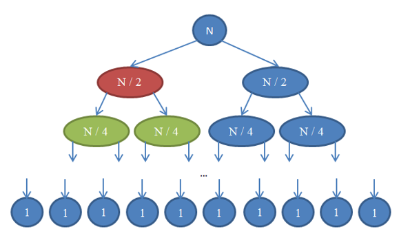
Let’s see what’s going on here. Each circle represents a call to the mergeSort function. The number written in the circle indicates the size of the array that is being sorted. The top blue circle is the original call to mergeSort, where we get to sort an array of size n. The arrows indicate recursive calls made between functions. The original call to mergeSort makes two calls to mergeSort on two arrays, each of size n / 2. This is indicated by the two arrows at the top. In turn, each of these calls makes two calls of its own to mergeSort two arrays of size n / 4 each, and so forth until we arrive at arrays of size 1. This diagram is called a recursion tree, because it illustrates how the recursion behaves and looks like a tree (the root is at the top and the leaves are at the bottom, so in reality it looks like an inversed tree). Notice that at each row in the above diagram, the total number of elements is n. To see this, take a look at each row individually. The first row contains only one call to mergeSort with an array of size n, so the total number of elements is n. The second row has two calls to mergeSort each of size n / 2. But n / 2 + n / 2 = n and so again in this row the total number of elements is n. In the third row, we have 4 calls each of which is applied on an n / 4-sized array, yielding a total number of elements equal to n / 4 + n / 4 + n / 4 + n / 4 = 4n / 4 = n. So again we getn elements. Now notice that at each row in this diagram the caller will have to perform a merge operation on the elements returned by the callees. For example, the circle indicated with red color has to sort n / 2 elements. To do this, it splits the n / 2-sized array into two n / 4-sized arrays, calls mergeSort recursively to sort those (these calls are the circles indicated with green color), then merges them together. This merge operation requires to merge n / 2 elements. At each row in our tree, the total number of elements merged is n. In the row that we just explored, our function merges n / 2 elements and the function on its right (which is in blue color) also has to merge n / 2 elements of its own. That yields n elements in total that need to be merged for the row we’re looking at. By this argument, the complexity for each row is Θ( n ). We know that the number of rows in this diagram, also called the depth of the recursion tree, will be log( n ). The reasoning for this is exactly the same as the one we used when analyzing the complexity of binary search. We have log( n ) rows and each of them is Θ( n ), therefore the complexity of mergeSort is Θ( n * log( n ) ). This is much better than Θ( n2 ) which is what selection sort gave us (remember that log( n ) is much smaller than n, and so n * log( n ) is much smaller than n * n = n2). If this sounds complicated to you, don’t worry: It’s not easy the first time you see it. Revisit this section and reread about the arguments here after you implement mergesort in your favourite programming language and validate that it works. As you saw in this last example, complexity analysis allows us to compare algorithms to see which one is better. Under these circumstances, we can now be pretty certain that merge sort will outperform selection sort for large arrays. This conclusion would be hard to draw if we didn’t have the theoretical background of algorithm analysis that we developed. In practice, indeed sorting algorithms of running time Θ( n * log( n ) ) are used. For example, the Linux kernel uses a sorting algorithm called heapsort, which has the same running time as mergesort which we explored here, namely Θ( n log( n ) ) and so is optimal. Notice that we have not proven that these sorting algorithms are optimal. Doing this requires a slightly more involved mathematical argument, but rest assured that they can’t get any better from a complexity point of view.

Searching/Sorting Algorithms, their asymptotic behavior and complexity analysis

Linear search on a list of n elements. In the worst case, the search must visit every element once. This happens when the value being searched for is either the last element in the list, or is not in the list. However, on average, assuming the value searched for is in the list and each list element is equally likely to be the value searched for, the search visits only n/2 elements. Insertion sort applied to a list of n elements, assumed to be all different and initially in random order. On average, half the elements in a list A1 … Aj are less than element Aj+1, and half are greater. Therefore the algorithm compares the j+1-st element to be inserted on the average with half the already sorted sub-list, so tj = j/2. Working out the resulting average-case running time yields a quadratic function of the input size, just like the worst-case running time. Quicksort applied to a list of n elements, again assumed to be all different and initially in random order. This popular sorting algorithm has an average-case performance of O(n log n), which contributes to making it a very fast algorithm in practice. But given a worst-case input, its performance degrades to O(n2).

Summary of the article Algorithmic complexity is concerned about how fast or slow particular algorithm performs. We define complexity as a numerical function T(n) - time versus the input size n. We want to define time taken by an algorithm without depending on the implementation details. But you agree that T(n) does depend on the implementation. A given algorithm will take different amounts of time on the same inputs depending on such factors as: processor speed; instruction set, disk speed, brand of compiler and etc. The way around is to estimate efficiency of each algorithm asymptotically. We will measure time T(n) as the number of elementary “steps” (defined in any way), provided each such step takes constant time.

Runtime Analysis One of the most important aspects of an algorithm is how fast it is. It is often easy to come up with an algorithm to solve a problem, but if the algorithm is too slow, it’s back to the drawing board. Since the exact speed of an algorithm depends on where the algorithm is run, as well as the exact details of its implementation, computer scientists typically talk about the runtime relative to the size of the input. For example, if the input consists of N integers, an algorithm might have a runtime proportional to N2, represented as O(N2). This means that if you were to run an implementation of the algorithm on your computer with an input of size N, it would take C*N2 seconds, where C is some constant that doesn’t change with the size of the input.

However, the execution time of many complex algorithms can vary due to factors other than the size of the input. For example, a sorting algorithm may run much faster when given a set of integers that are already sorted than it would when given the same set of integers in a random order. As a result, you often hear people talk about the worst-case runtime, or the average-case runtime. The worst-case runtime is how long it would take for the algorithm to run if it were given the most insidious of all possible inputs. The average-case runtime is the average of how long it would take the algorithm to run if it were given all possible inputs. Of the two, the worst-case is often easier to reason about, and therefore is more frequently used as a benchmark for a given algorithm. The process of determining the worst-case and average-case runtimes for a given algorithm can be tricky, since it is usually impossible to run an algorithm on all possible inputs.

The goal of computational complexity is to classify algorithms according to their performances. We will represent the time function T(n) using the “big-O” notation to express an algorithm runtime complexity. For example, the following statement T(n) = O(n2) says that an algorithm has a quadratic time complexity. For any monotonic functions f(n) and g(n) from the positive integers to the positive integers, we say that f(n) = O(g(n)) when there exist constants c > 0 and n0 > 0 such that f(n) ≤ c * g(n), for all n ≥ n0 Intuitively, this means that function f(n) does not grow faster than g(n), or that function g(n) is an upper bound for f(n), for all sufficiently large n→∞

Examples: • 1 = O(n) • n = O(n2) • log(n) = O(n) • 2 n + 1 = O(n) The “big-O” notation is not symmetric: n = O(n2) but n2 ≠ O(n). Exercise. Let us prove n2 + 2 n + 1 = O(n2). We must find such c and n0 that n 2 + 2 n + 1 ≤ c*n2. Let n0=1, then for n ≥ 1 1 + 2 n + n2 ≤ n + 2 n + n2 ≤ n2 + 2 n2 + n 2 = 4 n2 Therefore, c = 4.

Constant Time: O(1) An algorithm is said to run in constant time if it requires the same amount of time regardless of the input size. Examples: • array: accessing any element • fixed-size stack: push and pop methods • fixed-size queue: enqueue and dequeue methods Linear Time: O(n) An algorithm is said to run in linear time if its time execution is directly proportional to the input size, i.e. time grows linearly as input size increases. Examples: • array: linear search, traversing, find minimum • ArrayList: contains method • queue: contains method Logarithmic Time: O(log n) An algorithm is said to run in logarithmic time if its time execution is proportional to the logarithm of the input size. Example: • binary search locate the element a in a sorted (in ascending order) array by first comparing a with the middle element and then (if they are not equal) dividing the array into two subarrays; if a is less than the middle element you repeat the whole procedure in the left subarray, otherwise - in the right subarray. The procedure repeats until a is found or subarray is a zero dimension. Note, log(n) < n, when n→∞. Algorithms that run in O(log n) does not use the whole input. Quadratic Time: O(n2) An algorithm is said to run in quadratic time if its time execution is proportional to the square of the input size. Examples: • bubble sort, selection sort, insertion sort

Definition of “big Omega” We need the notation for the lower bound. A capital omega Ω notation is used in this case. We say that f(n) = Ω(g(n)) when there exist constant c that f(n) ≥ c*g(n) for for all sufficiently large n. Examples • n = Ω(1) • n2 = Ω(n) • n2 = Ω(n log(n)) • 2 n + 1 = O(n)

Definition of “big Theta” To measure the complexity of a particular algorithm, means to find the upper and lower bounds. A new notation is used in this case. We say that f(n) = Θ(g(n)) if and only f(n) = O(g(n)) and f(n) = Ω(g(n)). Examples • 2 n = Θ(n) • n2 + 2 n + 1 = Θ( n2)

Example. Let us consider an algorithm of sequential searching in an array.of size n. Its worst-case runtime complexity is O(n) Its best-case runtime complexity is O(1) Its average case runtime complexity is O(n/2)=O(n)

Approximate completion time for algorithms, N = 100

Common Algorithms and their practical usage

This document describes some common algorithms used in the IT industry and their brief explanations.

In Computer Science everything is an instruction and a step by step procedure to perform these instructions is an Algorithm. In other words an algorithm is a brief planning of how the problem in computer science will be solved in general. Therefore it is of major concern in the Computer Science world and almost every aspect of Computer Science need Algorithm. The following list include various algorithms used in Computer Science areas and a brief description about them.

Definition of algorithms Though I’ve defined it a numerous times in my previous articles also, but this time it again needs an exhaustive explanation and a computer science specific proper definition.

In computer systems, an algorithm is basically an instance of logic written in software by software developers to be effective for the intended “target” computer(s) for the target machines to produce output from given input (perhaps null). In simpler words “an algorithm is any well-defined computational procedure that takes some value, or set of values, as input and produces some value, or set of values as output.” Algorithms are like road maps for accomplishing a given, well-defined task. So, a chunk of code that calculates the terms of the Fibonacci sequence is an implementation of a particular algorithm. Even a simple function for adding two numbers is an algorithm in a sense, albeit a simple one.

Now there are many predefined algorithms which are commonly used to solve computers related problems and to devise more complexer algorithms. These algorithms acts as a foundation for making newer and complexer algorithms to solve specific problems.

Like divide and conquer algorithms, greedy approach towards a problem, backtracking, dynamic programming, recursion and randomized algorithms and many more. A brief explanation about each of these algorithms is given below.

Divide and Conquer (D&C) Like Greedy and Dynamic Programming, Divide and Conquer is an algorithmic paradigm. A typical Divide and Conquer algorithm solves a problem using following three steps.

1. Divide: Break the given problem into subproblems of same type.
2. Conquer: Recursively solve these subproblems
3. Combine: Appropriately combine the answers

Some common examples where D&C approach can be applied: – Finding a counterfeit coin using weight balance – Defective chess board – finding the kth smallest element

Some standard algorithms that are Divide and Conquer algorithms. • Binary search is a searching algorithm. In each step, the algorithm compares the input element x with the value of the middle element in array. If the values match, return the index of middle. Otherwise, if x is less than the middle element, then the algorithm recurs for left side of middle element, else recurs for right side of middle element.

• Quick sort is a sorting algorithm. The algorithm picks a pivot element, rearranges the array elements in such a way that all elements smaller than the picked pivot element move to left side of pivot, and all greater elements move to right side. Finally, the algorithm recursively sorts the subarrays on left and right of pivot element.

• Merge Sort is also a sorting algorithm. The algorithm divides the array in two halves, recursively sorts them and finally merges the two sorted halves.

• Closest Pair of Points The problem is to find the closest pair of points in a set of points in x-y plane. The problem can be solved in O(n^2) time by calculating distances of every pair of points and comparing the distances to find the minimum. The Divide and Conquer algorithm solves the problem in O(nLogn) time.

• Strassen’s Algorithm is an efficient algorithm to multiply two matrices. A simple method to multiply two matrices need 3 nested loops and is O(n^3). Strassen’s algorithm multiplies two matrices in O(n^2.8974) time.

• Cooley–Tukey Fast Fourier Transform (FFT) algorithm is the most common algorithm for FFT. It is a divide and conquer algorithm which works in O(nlogn) time.

• Karatsuba algorithm for fast multiplication it does multiplication of two n-digit numbers in at most

Greedy Approach Greedy is an algorithmic paradigm that builds up a solution piece by piece, always choosing the next piece that offers the most obvious and immediate benefit. Greedy algorithms are used for optimization problems. An optimization problem can be solved using Greedy if the problem has the following property: At every step, we can make a choice that looks best at the moment, and we get the optimal solution of the complete problem. If a Greedy Algorithm can solve a problem, then it generally becomes the best method to solve that problem as the Greedy algorithms are in general more efficient than other techniques like Dynamic Programming. But Greedy algorithms cannot always be applied. For example, Fractional Knapsack problem can be solved using Greedy, but 0-1 Knapsack cannot be solved using Greedy.

Some standard algorithms that are Greedy algorithms. • Kruskal’s Minimum Spanning Tree (MST): In Kruskal’s algorithm, we create a MST by picking edges one by one. The Greedy Choice is to pick the smallest weight edge that doesn’t cause a cycle in the MST constructed so far.

• Prim’s Minimum Spanning Tree: In Prim’s algorithm also, we create a MST by picking edges one by one. We maintain two sets: set of the vertices already included in MST and the set of the vertices not yet included. The Greedy Choice is to pick the smallest weight edge that connects the two sets.

• Dijkstra’s Shortest Path: The Dijkstra’s algorithm is very similar to Prim’s algorithm. The shortest path tree is built up, edge by edge. We maintain two sets: set of the vertices already included in the tree and the set of the vertices not yet included. The Greedy Choice is to pick the edge that connects the two sets and is on the smallest weight path from source to the set that contains not yet included vertices.

• Huffman Coding: Huffman Coding is a loss-less compression technique. It assigns variable length bit codes to different characters. The Greedy Choice is to assign least bit length code to the most frequent character.

The greedy algorithms are sometimes also used to get an approximation for Hard optimization problems. For example, Traveling Salesman Problem is a NP Hard problem. A Greedy choice for this problem is to pick the nearest unvisited city from the current city at every step. This solutions doesn’t always produce the best optimal solution, but can be used to get an approximate optimal solution.

Dynamic Programming (DP)

Dynamic Programming is an algorithmic paradigm that solves a given complex problem by breaking it into subproblems and stores the results of subproblems to avoid computing the same results again. Following are the two main properties of a problem that suggest that the given problem can be solved using Dynamic programming. 1) Overlapping Subproblems 2) Optimal Substructure

Overlapping Subproblems: Like Divide and Conquer, Dynamic Programming combines solutions of sub-problems. Dynamic Programming is mainly used when solutions of same subproblems are needed again and again. In dynamic programming, computed solutions of subproblems are stored in a table so that these don’t have to recomputed. So Dynamic Programming is not useful when there are no common (overlapping) subproblems because there is no point storing the solutions if they are not needed again. For example, Binary Search doesn’t have common subproblems. If we take example of following recursive program for Fibonacci Numbers, there are many subproblems which are solved again and again.

/* simple recursive program for Fibonacci numbers */ int fib(int n) { if ( n <= 1 ) return n; return fib(n-1) + fib(n-2); }

Recursion tree for execution of fib(5)

                     fib(5)
                 /             \
           fib(4)                fib(3)
         /      \                /     \
     fib(3)      fib(2)         fib(2)    fib(1)
    /     \        /    \       /    \   fib(2)   fib(1)  fib(1) fib(0) fib(1) fib(0)   /    \ fib(1) fib(0)

We can see that the function f(3) is being called 2 times. If we would have stored the value of f(3), then instead of computing it again, we would have reused the old stored value. There are following two different ways to store the values so that these values can be reused.

a) Memoization (Top Down): b) Tabulation (Bottom Up):

Memoization (Top Down): The memoized program for a problem is similar to the recursive version with a small modification that it looks into a lookup table before computing solutions. We initialize a lookup array with all initial values as NIL. Whenever we need solution to a subproblem, we first look into the lookup table. If the precomputed value is there then we return that value, otherwise we calculate the value and put the result in lookup table so that it can be reused later.

Tabulation (Bottom Up): The tabulated program for a given problem builds a table in bottom up fashion and returns the last entry from table.

Both tabulated and Memoized store the solutions of subproblems. In Memoized version, table is filled on demand while in tabulated version, starting from the first entry, all entries are filled one by one. Unlike the tabulated version, all entries of the lookup table are not necessarily filled in memoized version. For example, memoized solution of LCS problem doesn’t necessarily fill all entries. To see the optimization achieved by memoized and tabulated versions over the basic recursive version, see the time taken by following runs for 40th Fibonacci number.

Backtracking

Recursion

Randomized Algorithms

Searching Algorithms Searching a sorted collection is a common task. A dictionary is a sorted list of word definitions. Given a word, one can find its definition. A telephone book is a sorted list of people’s names, addresses, and telephone numbers. Knowing someone’s name allows one to quickly find their telephone number and address. If the list to be searched contains more than a few items (a dozen, say) a binary search will require far fewer comparisons than a linear search, but it imposes the requirement that the list be sorted. Similarly, a hash search can be faster than a binary search but imposes still greater requirements. If the contents of the array are modified between searches, maintaining these requirements may even take more time than the searches. And if it is known that some items will be searched for much more often than others, and it can be arranged that these items are at the start of the list, then a linear search may be the best. So the choice of searching algorithm to be used depends upon various conditions as we can easily observe from the above discussed cases that every practical problem have different demands and to take care of all such requirements, specific modifications are made in the general searching algorithm.

Dictionary search/predictive search

Selection algorithm: Finds the kth largest item in a list

Binary search algorithm: Locates an item in a sorted list Also called half-interval search A binary search halves the number of items to check with each iteration, so locating an item (or determining its absence) takes logarithmic time. A binary search is a dichotomic divide and conquer search algorithm. Binary Search can be implmented either recursively or iterativly.

Breadth-first search: Traverses a graph level by level

Depth-first search: Traverses a graph branch by branch

Best-first search: Traverses a graph in the order of likely importance using a priority queue

tree search: Special case of best-first search that uses heuristics to improve speed

Uniform-cost search: A tree search that finds the lowest cost route where costs vary

Predictive search

Binary like search: which factors in magnitude of search term versus the high and low values in the search

Hash table: Associate keys to items in an unsorted collection, to retrieve them in a linear time

Interpolated search: See predictive search

Sorting Algorithms Sorting provides a good example of an algorithm that is very frequently used by computer scientists. The simplest way to sort a group of items is to start by removing the smallest item from the group, and put it first. Then remove the next smallest, and put it next and so on. Unfortunately, this algorithm is O(N2), meaning that the amount of time it takes is proportional to the number of items squared. If you had to sort a billion things, this algorithm would take around 1018 operations. To put this in perspective, a desktop PC can do a little bit over 109 operations per second, and would take years to finish sorting a billion things this way.

Luckily, there are a number of better algorithms (quicksort, heapsort and mergesort, for example) that have been devised over the years, many of which have a runtime of O(N * Log(N)). This brings the number of operations required to sort a billion items down to a reasonable number that even a cheap desktop could perform. Instead of a billion squared operations (1018) these algorithms require only about 10 billion operations (1010), a factor of 100 million faster. Some algorithms (selection, bubble, heapsort) work by moving elements to their final position, one at a time. You sort an array of size N, put 1 item in place, and continue sorting an array of size N–1 (heapsort is slightly different). Some algorithms (insertion, quicksort, counting, radix) put items into a temporary position, close(r) to their final position. You rescan, moving items closer to the final position with each iteration. One technique is to start with a “sorted list” of one element, and merge unsorted items into it, one at a time.

Binary tree sort: Sort of a binary tree, incremental, similar to insertion sort.

Bogosort: Inefficient random sort of a desk card.

Bubble sort: For each pair of indices, swap the items if out of order. [Best: O(n), Worst:O(N^2)] Starting on the left, compare adjacent items and keep “bubbling” the larger one to the right (it’s in its final place). Bubble sort the remaining N -1 items. With bubble-sort, either you bubble items “forward” (left-to-right) and move the endpoint backwards (decreasing), or bubble items “backward” (right-to-left) and increase the left endpoint. Either way, some index is decreasing. You also need to keep track of the next-to-last endpoint, so you don’t swap with a non-existant item.

Bucket sort: Split a list in buckets and sort them individually. Generalized pigeonhole sort:

Cocktail sort (or bidirectional bubble, shaker, ripple, shuttle, happy hour sort): Variation of bubble sort that sorts in both directions each pass through the list.

Comb sort: Efficient variation of bubble sort that eliminates “turtles”, the small values near the end of the list and makes use of gaps bewteen values.

Counting sort: It uses the range of numbers in the list A to create an array B of this length. Indexes in B are used to count how many elements in A have a value less than i. Counting sort [Best/Avg/Worst: O(N)] Assuming the data are integers, in a range of 0-k. Create an array of size K to keep track of how many items appear (3 items with value 0, 4 items with value 1, etc). Given this count, you can tell the position of an item — all the 1′s must come after the 0′s, of which there are 3. Therefore, the 1′s start at item #4. Thus, we can scan the items and insert them into their proper position. • Creating the count array is O(N) • Inserting items into their proper position is O(N) • I oversimplified here — there is a summation of the counts, and a greatest-to-least ordering which keeps the sort stable.

Gnome sort: Similar to insertion sort except that moving an element to its proper place is accomplished by a series of swaps, as in bubble sort.

Heapsort: Convert the list into a heap, keep removing the largest element from the heap and adding it to the end of the list. Heapsort [Best/Avg/Worst: O(N lg N)] Add all items into a heap. Pop the largest item from the heap and insert it at the end (final position). Repeat for all items. • Heapsort is just like selection sort, but with a better way to get the largest element. Instead of scanning all the items to find the max, it pulls it from a heap. Heaps have properties that allow heapsort to work in-place, without additional memory. • Creating the heap is O(N lg N). Popping items is O(1), and fixing the heap after the pop is lgN. There are N pops, so there is another O(N lgN) factor, which is O(N lg N) overall. • Heapsort has O(N lgN) behavior, even in the worst case, making it good for real-time applications

Insertion sort: Determine where the current item belongs in the list of sorted ones, and insert it there. Insertion Sort [Best: O(N), Worst:O(N^2)] Start with a sorted list of 1 element on the left, and N-1 unsorted items on the right. Take the first unsorted item (element #2) and insert it into the sorted list, moving elements as necessary. We now have a sorted list of size 2, and N -2 unsorted elements. Repeat for all elements. • Like bubble sort, I found this counter-intuitive because you step “backwards” • This is a little like bubble sort for moving items, except when you encounter an item smaller than you, you stop. If the data is reverse-sorted, each item must travel to the head of the list, and this becomes bubble-sort. • There are various ways to move the item leftwards — you can do a swap on each iteration, or copy each item over its neighbor

Introsort Or introspective sort: It begins in quicksort and switches to heapsort at certain recursion level.

Merge sort: Sort the first and second half of the list separately, then merge the sorted lists.

Pancake sort: Reverse elements of some prefix of a sequence.

Pigeonhole sort: Fill an empty array with all elements of an array to be sorted, in order.

Postman sort: Hierarchical variant of bucket sort, used by post offices.

Quicksort: Divide list into two, with all items on the first list coming before all items on the second list.; then sort the two lists. Often the method of choice. Quicksort [Best: O(N lg N), Avg: O(N lg N), Worst:O(N^2)] There are may versions of Quicksort, which is one of the most popular sorting methods due to its speed (O(N lgN) average, but O(N^2) worst case). Here’s a few: Using external memory: • Pick a “pivot” item • Partition the other items by adding them to a “less than pivot” sublist, or “greater than pivot” sublist • The pivot goes between the two lists • Repeat the quicksort on the sublists, until you get to a sublist of size 1 (which is sorted). • Combine the lists — the entire list will be sorted Using in-place memory: • Pick a pivot item and swap it with the last item. We want to partition the data as above, and need to get the pivot out of the way. • Scan the items from left-to-right, and swap items greater than the pivot with the last item (and decrement the “last” counter). This puts the “heavy” items at the end of the list, a little like bubble sort. • Even if the item previously at the end is greater than the pivot, it will get swapped again on the next iteration. • Continue scanning the items until the “last item” counter overlaps the item you are examining – it means everything past the “last item” counter is greater than the pivot. • Finally, switch the pivot into its proper place. We know the “last item” counter has an item greater than the pivot, so we swap the pivot there. • Phew! Now, run quicksort again on the left and right subset lists. We know the pivot is in its final place (all items to left are smaller; all items to right are larger) so we can ignore it. Using in-place memory w/two pointers: • Pick a pivot and swap it out of the way • Going left-to-right, find an oddball item that is greater than the pivot • Going right-to-left, find an oddball item that is less than the pivot • Swap the items if found, and keep going until the pointers cross — re-insert the pivot • Quicksort the left and right partitions • Note: this algorithm gets confusing when you have to keep track of the pointers and where to swap in the pivot Notes • If a bad pivot is chosen, you can imagine that the “less” subset is always empty. That means we are only creating a subset of one item smaller each time, which gives us O(N^2) behavior in the worst case. • If you choose the first item, it may be the smallest item in a sorted list and give worst-case behavior. You can choose a random item, or median-of-three (front, middle, end). • Quicksort is fast because it uses spatial locality — it walks neighboring elements, comparing them to the pivot value (which can be stored in a register). It makes very effective use of caching. • The pivot is often swapped to the front, so it is out of the way during the pivotting. Afterwards, it is swapped into place (with a pivot item that is less than or equal to it, so the pivot is preservd). • The quicksort algorithm is complicated, and you have to pass left and right boundary variables

Radix sort: Sorts keys associated to items, or integer by processing digits. Radix sort [Best/Avg/Worst: O(N)] Get a series of numbers, and sort them one digit at a time (moving all the 1000′s ahead of the 2000′s, etc.). Repeat the sorting on each set of digits. • Radix sort uses counting sort for efficient O(N) sorting of the digits (k = 0…9) • Actually, radix sort goes from least significant digit (1′s digit) to most significant, for reasons I’ll explain later (see CLRS book) • Radix & counting sort are fast, but require structured data, external memory and do not have the caching benefits of quicksort.

Selection sort: Pick the smallest of the remaining elements, add it to the end of the sorted list. Selection Sort [Best/Worst: O(N^2)] Scan all items and find the smallest. Swap it into position as the first item. Repeat the selection sort on the remaining N-1 items. • I found this the most intuitive and easiest to implement — you always iterate forward (i from 0 to N-1), and swap with the smallest element (always i).

Shell sort: Improves insertion sort with use of gaps between values.

Smoothsort: See heapsort.

Stochastic sort: See bogosort.

Automata

Powerset construction. Algorithm to convert non deterministic automaton to deterministic automaton. Todd-Coxeter algorithm. Procedure for generating cosets.

Artificial intelligence

Alpha-beta. Alpha max plus beta min. Widely used in board games. Ant-algorithms. The ant colony optimisation is a set of algorithms inspired by ant behavior to solve a problem, find the best path between two locations. DE (Differential evolution). Solve the Chebyshev polynomial fitting problem. Semi-Supervised Recognition of Sarcastic Sentences in Online Product Reviews. Algortithm that recognize sacarsms or irony in a tweet or an online document. A such algorithm will be essential for humanoid robots programming too.

Computer vision

Epitome. Represent an image or video by a smaller one. Counting objects in an image. Uses the connected-component labeling algorithm to first label each object, and count then the objects. O’Carroll algorithm. From a mathematical conversion of insect vision, this algorithm evaluates how to get around avoiding objects.

Genetic algorithms

They uses three operator. selection (choose solution), reproduction (use choosen solutions to construct other ones), replacement (replace solution if better).

Fitness proportionate selection. Also known as roulette-wheel selection, is a function used for selecting solutions. Truncation selection. Another method for selecting solutions, ordered by fitness. Tournament selection. Select the best solution by a kind of tournament. Stochastic universal sampling. The individuals are mapped to contiguous segments of a line, such that each individual’s segment is equal in size to its fitness exactly as in roulette-wheel selection.

Neural networks

Hopfield net. Recurrent artificial neural network that serve as content-addressable memory systems with binary threshold units. They converge to a stable state. Backpropagation. Supervised learning technique used for training artificial neural networks. Self-organizing map (Kohonen map). Neural networks trained using unsupervised learning to produce low dimensional (2D, 3D) representation of the training samples. Good for visualizing high-dimensional data.

Bioinformatics

Needleman-Wunsch. Performs a global alignment on two sequences, for protein or nucleotide sequences. Smith-Waterman. Variation of the Needleman-Wunsch.

Compression

Lossless compression algorithms

Burrows-Wheeler transform. Preprocessing useful for improving lossless compression. Deflate. Data compression used by ZIP. Delta encoding. Aid to compression of data in which sequential data occurs frequently. Incremental encoding. Delta encoding applied to sequences of strings. LZW. (Lempel-Ziv-Welch). Successor of LZ78. Builds a translation table from the data to compress. Is used by the GIF graphical format. LZ77 and 78. The basis of further LZ variations (LZW, LZSS, …). They are both dictionary coders. LZMA. Short for Lempel-Ziv-Markov chain-Algorithm. LZO. Data compression algorithm that is focused on speed. PPM (Prediction by Partial Matching). Adaptive statistical data compression technique based on context modeling and prediction. Shannon-Fano coding. Constructs prefix codes based on a set of symbols and their probabilities. Truncated binary. An entropy encoding typically used for uniform probability distributions with a finite alphabet. Improve binary encoding. Run-length encoding. Primary compression that replaces a sequence of same code by the number of occurences. Sequitur. Incremental grammar inference on a string. EZW (Embedded Zerotree Wavelet). Progressive encoding to compress an image into a bit stream with increasing accuracy. May be lossy compression also with better results.

Entropy encoding Coding scheme that assigns codes to symbols so as to match code lengths with the probabilities of the symbols .

Huffman coding. Simple lossless compression taking advantage of relative character frequencies. Adaptive Huffman coding. Adaptive coding technique based on Huffman coding. Arithmetic coding. Advanced entropy coding. Range encoding. Same as arithmetic coding, but looked at in a slightly different way. Unary coding. Code that represents a number n with n ones followed by a zero. Elias delta, gamma, omega coding. Universal code encoding the positive integers. Fibonacci coding. Universal code which encodes positive integers into binary code words. Golomb coding. Form of entropy coding that is optimal for alphabets following geometric distributions. Rice coding. Form of entropy coding that is optimal for alphabets following geometric distributions.

Lossy compression algorithms

Linear predictive coding. Lossy compression by representing the spectral envelope of a digital signal of speech in compressed form. A-law algorithm. Standard companding algorithm. Mu-law algorithm. Standard analog signal compression or companding algorithm. Fractal compression. Method used to compress images using fractals. Transform coding. Type of data compression for data like audio signals or photographic images. Vector quantization. Technique often used in lossy data compression. Wavelet compression. Form of data compression well suited for image and audio compression.

Cryptography

Secret key (symmetric encryption)

Use a secret key (or a pair of directly related keys) for both decryption and encryption.

Advanced Encryption Standard (AES), also known as Rijndael. Blowfish. Designed by Schneier as a general-purpose algorithm, intended as a replacement for the aging DE. Data Encryption Standard (DES), formerly DE Algorithm. IDEA (International Data Encryption Algorithm). Formerly IPES (Improved PES), another replacement for DES. Is used by PGP (Pretty Good Privacy). Performs transformations on data splitted in blocks, using a key. RC4 or ARC4. Stream cipher widely-used in protocols such as SSL for Internet traffic and WEP for wireless networks. Tiny Encryption Algorithm. Easy to implement block cipher algorithme using some formulas. PES (Proposed Encryption Standard). Older name for IDEA.

Public key (asymmetric encryption)

Use a pair of keys, designated as public key and private key. The public key encrypt the message, only the private key permits to decrypt it.

DSA (Digital Signature Algorithm). Generate keys with prime and random numbers. Was used by US agencies, and now public domain. ElGamal. Based on Diffie-Hellman, used by GNU Privacy Guard software, PGP, and other cryptographic systems. RSA (Rivest, Shamir, Adleman). Widely used in electronic commerce protocols. Use prime numbers. Diffie-Hellman (Merkle) key exchange (or exponential key exchange). Method and algorithm to share secret over an unprotected communications channel. Used by RSA. NTRUEncrypt. Make use of rings of polynomials with convolution multiplications.

Message digest functions

A message digest is a code resulting of the encryption of a string or data of any length, processed by a hash function.

MD5. Used for checking ISO images of CDs or DVDs. RIPEMD (RACE Integrity Primitives Evaluation Message Digest). Based upon the principles of MD4 and similar to SHA-1. SHA-1 (Secure Hash Algorithm 1). Most commonly used of the SHA set of related cryptographic hash functions. Was designed by the NSA agency. HMAC. keyed-hash message authentication. Tiger (TTH). Usually used in Tiger tree hashes.

Cryptographic using pseudo-random numbers See. Random Number Generators

Techniques in cryptography

Secret sharing, Secret Splitting, Key Splitting, M of N algorithms.

Shamir’s secret sharing scheme. This is a formula based on polynomial interpolation. Blakley’s secret sharing scheme. Is geometric in nature, the secret is a point in an m-dimensional space.

Other techniques and decryption

Subset sum. Given a set of integers, does any subset sum equal zero? Used in cryptography. Shor’s algorithm. Quantum algorithm able to decrypt a code based on asymetric functions such as RSA.

Geometry

Gift wrapping. Determining the convex hull of a set of points. Gilbert-Johnson-Keerthi distance. Determining the smallest distance between two convex shapes. Graham scan. Determining the convex hull of a set of points in the plane. Line segment intersection. Finding whether lines intersect with a sweep line algorithm. Point in polygon. Tests whether a given point lies within a given. Ray/Plane intersection. Line/Triangle intersection. Particular case of Ray/Plane intersection. Polygonization of implicit surfaces. Approximate an implicit surface with a polygonal representation. Triangulation. Method to evaluate the distance to a point from angles to other points, whose distance is known.

Graphs 3D Surface Tracker Technology. Process to add images on walls in a video while hidden surfaces are taken into account. Bellman-Ford. Computes shortest paths in a weighted graph (where some of the edge weights may be negative). Dijkstra’s algorithm. Computes shortest paths in a graph with non-negative edge weights. Perturbation methods. An algorithm that computes a locally shortest paths in a graph. Floyd-Warshall. Solves the all pairs shortest path problem in a weighted, directed graph. Floyd’s cycle-finding. Finds cycles in iterations. Johnson. All pairs shortest path algorithm in sparse weighted directed graph. Kruskal. Finds a minimum spanning tree for a graph. Prim’s. Finds a minimum spanning tree for a graph. Also called DJP , Jarník or Prim–Jarník algorithm. Boruvka. Finds a minimum spanning tree for a graph. Ford-Fulkerson. Computes the maximum flow in a graph. Edmonds-Karp. Implementation of Ford-Fulkerson. Nonblocking Minimal Spanning Switch. For a telephone exchange. Woodhouse-Sharp. Finds a minimum spanning tree for a graph. Spring based. Algorithm for graph drawing. Hungarian. Algorithm for finding a perfect matching. Coloring algorithm. Graph coloring algorithm. Nearest neighbour. Find nearest neighbour. Topological sort. Sort a directed acyclic graph in such a manner that each node comes before all nodes to which it has edges (according to directions). Tarjan’s off-line least common ancestors algorithm. Compute lowest common ancestors for pairs of nodes in a tree.

Graphics

Bresenham’s line algorithm. Uses decision variables to plots a straight line between 2 specified points. Landscape Draw a 3D scenery. DDA line algorithm. Uses floating-point math to plots a straight line between 2 specified points. Flood fill. Fills a connected region with a color. Image Restoring. Restore photo, improve images. Xiaolin Wu’s line algorithm. Line antialiasing. Painter’s algorithm. Detects visible parts of a 3-dimensional scenery. Ray tracing. Realistic image rendering. Phong shading. An illumination model and an interpolation method in 3D computer graphics. Gouraud shading. Simulate the differing effects of light and colour across the surface of a 3D object. Scanline rendering. Constructs an image by moving an imaginary line. Global illumination. Considers direct illumination and reflection from other objects. Interpolation. Constructing new data points such as in digital zoom. Resynthesizer. Remove an object on a photo and rebuild the background Used by Photoshop and The Gimp. Resynthesizer tutorial . Slope-intercept algorithm. It is an implementation of the slope-intercept formula for drawing a line. Spline interpolation. Reduces error with Runge’s phenomenon. 3D Surface Tracker Technology. Adding images or vidéo on walls in a vidéo, hidden surfaces being taken into account.

Shortest Path

Algorithms for finding the shortest path from one point to another have been researched for years. Applications abound, but lets keep things simple by saying we want to find the shortest path from point A to point B in a city with just a few streets and intersections. There are quite a few different algorithms that have been developed to solve such problems, all with different benefits and drawbacks. Before we delve into them though, lets consider how long a naive algorithm - one that tries every conceivable option - would take to run. If the algorithm considered every possible path from A to B (that didn’t go in circles), it would not finish in our lifetimes, even if A and B were both in a small town. The runtime of this algorithm is exponential in the size of the input, meaning that it is O(CN) for some C. Even for small values of C, CN becomes astronomical when N gets even moderately large.

One of the fastest algorithms for solving this problem has a runtime of O(EVLog(V)), where E is the number of road segments, and V is the number of intersections. To put this in perspective, the algorithm would take about 2 seconds to find the shortest path in a city with 10,000 intersections, and 20,000 road segments (there are usually about 2 road segments per intersection). The algorithm, known as Djikstra’s Algorithm, is fairly complex, and requires the use of a data structure known as a priority queue. In some applications, however, even this runtime is too slow (consider finding the shortest path from New York City to San Francisco - there are millions of intersections in the US), and programmers try to do better by using what are known as heuristics. A heuristic is an approximation of something that is relevant to the problem, and is often computed by an algorithm of its own. In the shortest path problem, for example, it is useful to know approximately how far a point is from the destination. Knowing this allows for the development of faster algorithms (such as A*, an algorithm that can sometimes run significantly faster than Djikstra’s algorithm) and so programmers come up with heuristics to approximate this value. Doing so does not always improve the runtime of the algorithm in the worst case, but it does make the algorithm faster in most real-world applications.

Approximate algorithms

Sometimes, however, even the most advanced algorithm, with the most advanced heuristics, on the fastest computers is too slow. In this case, sacrifices must be made that relate to the correctness of the result. Rather than trying to get the shortest path, a programmer might be satisfied to find a path that is at most 10% longer than the shortest path.

In fact, there are quite a few important problems for which the best-known algorithm that produces an optimal answer is insufficiently slow for most purposes. The most famous group of these problems is called NP, which stands for non-deterministic polynomial (don’t worry about what that means). When a problem is said to be NP-complete or NP-hard, it mean no one knows a good way to solve them optimally. Furthermore, if someone did figure out an efficient algorithm for one NP-hard problem, that algorithm would be applicable to all NP-hard problems.

A good example of an NP-hard problem is the famous traveling salesman problem. A salesman wants to visit N cities, and he knows how long it takes to get from each city to each other city. The question is “how fast can he visit all of the cities?” Since the fastest known algorithm for solving this problem is too slow - and many believe this will always be true - programmers look for sufficiently fast algorithms that give good, but not optimal solutions.

Random Algorithms

Yet another approach to some problems is to randomize an algorithm is some way. While doing so does not improve the algorithm in the worst case, it often makes very good algorithms in the average case. Quicksort is a good example of an algorithm where randomization is often used. In the worst case, quicksort sorts a group of items in O(N2), where N is the number of items. If randomization is incorporated into the algorithm, however, the chances of the worst case actually occurring become diminishingly small, and on average, quicksort has a runtime of O(NLog(N)). Other algorithms guarantee a runtime of O(NLog(N)), even in the worst case, but they are slower in the average case. Even though both algorithms have a runtime proportional to NLog(N), quicksort has a smaller constant factor - that is it requires CNLog(N) operations, while other algorithms require more like 2CNLog(N) operations.

Another algorithm that uses random numbers finds the median of a group of numbers with an average runtime of O(N). This is a significant improvement over sorting the numbers and taking the middle one, which takes O(N*Log(N)). Furthermore, while deterministic (non-random) algorithms exist for finding the median with a runtime of O(N), the random algorithm is attractively simple, and often faster than the deterministic algorithms.

The basic idea of the median algorithm is to pick one of the numbers in the group at random, and count how many of the numbers in the group are less than it. Lets say there are N numbers, and K of them are less than or equal to the number we picked at random. If K is less than half of N, then we know that the median is the (N/2-K) th number that is greater than the random number we picked, so we discard the K numbers less than or equal to the random number. Now, we want to find the (N/2-K) th smallest number, instead of the median. The algorithm is the same though, and we simply pick another number at random, and repeat the above steps.

Compression

Another class of algorithm deals with situations such as data compression. This type of algorithm does not have an expected output (like a sorting algorithm), but instead tries to optimize some other criteria. In the case of data compression, the algorithm (LZW, for instance) tries to make the data use as few bytes as possible, in such a way that it can be decompressed to its original form. In some cases, this type of algorithm will use the same techniques as other algorithms, resulting in output that is good, but potentially sub-optimal. JPG and MP3 compression, for example, both compress data in a way that makes the final result somewhat lower quality than the original, but they create much smaller files. MP3 compression does not retain every feature of the original song file, but it attempts to maintain enough of the details to capture most of the quality, while at the same time ensuring the significantly reduced file size that we all know and love. The JPG image file format follows the same principle, but the details are significantly different since the goal is image rather than audio compression.

The Importance of Knowing Algorithms

As a computer scientist, it is important to understand all of these types of algorithms so that one can use them properly. If you are working on an important piece of software, you will likely need to be able to estimate how fast it is going to run. Such an estimate will be less accurate without an understanding of runtime analysis. Furthermore, you need to understand the details of the algorithms involved so that you’ll be able to predict if there are special cases in which the software won’t work quickly, or if it will produce unacceptable results.

Of course, there are often times when you’ll run across a problem that has not been previously studied. In these cases, you have to come up with a new algorithm, or apply an old algorithm in a new way. The more you know about algorithms in this case, the better your chances are of finding a good way to solve the problem. In many cases, a new problem can be reduced to an old problem without too much effort, but you will need to have a fundamental understanding of the old problem in order to do this.

As an example of this, lets consider what a switch does on the Internet. A switch has N cables plugged into it, and receives packets of data coming in from the cables. The switch has to first analyze the packets, and then send them back out on the correct cables. A switch, like a computer, is run by a clock with discrete steps - the packets are send out at discrete intervals, rather than continuously. In a fast switch, we want to send out as many packets as possible during each interval so they don’t stack up and get dropped. The goal of the algorithm we want to develop is to send out as many packets as possible during each interval, and also to send them out so that the ones that arrived earlier get sent out earlier. In this case it turns out that an algorithm for a problem that is known as “stable matching” is directly applicable to our problem, though at first glance this relationship seems unlikely. Only through pre-existing algorithmic knowledge and understanding can such a relationship be discovered.

More Real-world Examples

Other examples of real-world problems with solutions requiring advanced algorithms abound. Almost everything that you do with a computer relies in some way on an algorithm that someone has worked very hard to figure out. Even the simplest application on a modern computer would not be possible without algorithms being utilized behind the scenes to manage memory and load data from the hard drive.

There are dozens of applications of complicated algorithms, but I’m going to discuss two problems that require the same skills as some past TopCoder problems. The first is known as the maximum flow problem, and the second is related to dynamic programming, a technique that often solves seemingly impossible problems in blazing speed.

Maximum Flow

The maximum flow problem has to do with determining the best way to get some sort of stuff from one place to another, through a network of some sort. In more concrete terms, the problem first arose in relation to the rail networks of the Soviet Union, during the 1950’s. The US wanted to know how quickly the Soviet Union could get supplies through its rail network to its satellite states in Eastern Europe.

In addition, the US wanted to know which rails it could destroy most easily to cut off the satellite states from the rest of the Soviet Union. It turned out that these two problems were closely related, and that solving the max flow problem also solves the min cut problem of figuring out the cheapest way to cut off the Soviet Union from its satellites.

The first efficient algorithm for finding the maximum flow was conceived by two Computer Scientists, named Ford and Fulkerson. The algorithm was subsequently named the Ford-Fulkerson algorithm, and is one of the more famous algorithms in computer science. In the last 50 years, a number of improvements have been made to the Ford-Fulkerson algorithm to make it faster, some of which are dauntingly complex.

Since the problem was first posed, many additional applications have been discovered. The algorithm has obvious relevance to the Internet, where getting as much data as possible from one point to another is important. It also comes up in many business settings, and is an important part of operations research. For example, if you have N employees and N jobs that need to be done, but not every employee can do every job, the max flow algorithm will tell you how to assign your N employees to jobs in such a way that every job gets done, provided that’s possible. Graduation, from SRM 200, is a good example of a TopCoder problem that lends itself to a solution using max flow.

Sequence comparison

Many coders go their entire careers without ever having to implement an algorithm that uses dynamic programming. However, dynamic programming pops up in a number of important algorithms. One algorithm that most programmers have probably used, even though they may not have known it, finds differences between two sequences. More specifically, it calculates the minimum number of insertions, deletions, and edits required to transform sequence A into sequence B.

For example, lets consider two sequences of letters, “AABAA” and “AAAB”. To transform the first sequence into the second, the simplest thing to do is delete the B in the middle, and change the final A into a B. This algorithm has many applications, including some DNA problems and plagiarism detection. However, the form in which many programmers use it is when comparing two versions of the same source code file. If the elements of the sequence are lines in the file, then this algorithm can tell a programmer which lines of code were removed, which ones were inserted, and which ones were modified to get from one version to the next.

Without dynamic programming, we would have to consider a - you guessed it - exponential number of transformations to get from one sequence to the other. As it is, however, dynamic programming makes for an algorithm with a runtime of only O(N*M), where N and M are the numbers of elements in the two sequences.

Conclusion

The different algorithms that people study are as varied as the problems that they solve. However, chances are good that the problem you are trying to solve is similar to another problem in some respects. By developing a good understanding of a large range of algorithms, you will be able to choose the right one for a problem and apply it properly. Furthermore, solving problems like those found in TopCoder’s competitions will help you to hone your skills in this respect. Many of the problems, though they may not seem realistic, require the same set of algorithmic knowledge that comes up every day in the real world.